A computational problem may begin as a simple mathematical expression but become computationally expensive when it has to be evaluated millions or billions of times.

For example, a researcher may need to:

• evaluate a function on a very fine grid;
• perform a numerical simulation;
• solve a differential equation;
• explore a large parameter space;
• perform Monte Carlo calculations;
• process large matrices;
• analyse large experimental datasets;
• generate high-resolution mathematical visualizations.

The important question is therefore not only:

“How powerful is the computer?”

but also:

“How can my mathematical computation be expressed so that the available hardware can execute it efficiently?”

Druta provides several levels of computational capability:

                                DRUTA
                                  |
                   +--------------+--------------+
                   |                             |
                  CPU                           GPU
                   |                             |
            +------+------+                    CUDA
            |             |                 parallelism
         Serial        OpenMP                    |
            |             |                      |
       one CPU        many CPU                many GPU
      execution       threads                 threads

The same mathematical problem may therefore have several possible implementations.

This tutorial uses the Mandelbrot set as a simple example because:

1. it is mathematically interesting;
2. it's computation can be visualized immediately;
3. each pixel can be calculated independently, making it a natural example of parallel computing.

For a programmer, the most relevant hardware features are the ones that affect how a program can execute.

2.1 CPU

Druta contains:

• 2 CPU sockets
• 12 physical cores per socket
• 24 physical CPU cores in total
• 48 logical processors through simultaneous multithreading

The distinction between physical and logical processors is important.

                         Druta CPU
                           2 sockets
                              |
                +-------------+-------------+
                |                           |
             Socket 0                    Socket 1
                |                           |
         12 physical cores          12 physical cores
                |                           |
                +-------------+-------------+
                              |
                      24 physical cores
               24 physical cores × 2 hardware
                      threads per core
                              |
                              v
                      48 logical CPUs

Therefore, saying that Druta can run 48 OpenMP threads does not mean that it has 48 physical CPU cores. It has 24 physical cores and 48 logical processors.

For a programmer, the CPU provides several possibilities:

This tutorial demonstrates the first two.

2.2 Main Memory

Druta has approximately 256 GB of RAM.

Large RAM is particularly useful for mathematical computing involving:

• large matrices;
• large simulation grids;
• image stacks;
• numerical datasets;
• finite-difference calculations;
• statistical computations;
• intermediate arrays.

Having a large amount of RAM does not automatically make a program fast.

A program may instead be limited by:

• CPU computation;
• memory bandwidth;
• storage;
• CPU-to-GPU data transfers;
• algorithmic dependencies.

The first step is therefore to understand what the computation actually needs.

2.3 GPU

Druta has an:

NVIDIA RTX 4500 Ada Generation

The CUDA experiment reports:

• 60 streaming multiprocessors (SMs);
• approximately 24 GB of GPU memory;
• CUDA execution using a 16 × 16 thread block.

A useful mental model is:

    CPU
     |
     +-- relatively small number of powerful CPU cores
     |
     +-- good for general-purpose work and complex control flow
    
    
    GPU
     |
     +-- many parallel execution units
     |
     +-- excellent for large numbers of similar calculations

The GPU does not automatically accelerate every program.

The algorithm must contain suitable parallelism, and the cost of moving data between CPU memory and GPU memory may also matter.

The Mandelbrot set is defined using the iteration

$$z_{n+1}=z_n^2+c$$

where

$$c=x+iy$$

and initially

$$z_0=0.$$

For every point $c$, we repeatedly calculate

$$z_1=c,$$

$$z_2=z_1^2+c,$$

$$z_3=z_2^2+c,$$

and so on.

A point is considered to have escaped when

$$|z_n|>2.$$

In an actual computer program, we stop when either:

1. the magnitude exceeds 2; or
2. a specified maximum number of iterations is reached.

The exact Mandelbrot set is defined by whether the sequence remains bounded. In a computer visualization, however, we perform only a finite number of iterations. The value of maxIter therefore determines the numerical approximation used to colour the image.

The number of iterations required before escape is used to determine the corresponding pixel value.

3.1 From Mathematics to Pixels

Suppose we want an image of width $W$ and height $H$.

Each pixel corresponds to one point

$$c=x+iy.$$

Conceptually:

for every pixel (px, py):
      convert pixel position to c = x + iy
      z = 0
      for iteration = 1 ... maxIterations:
          z = z*z + c
          if |z| > 2:
              break
      store iteration count

The important observation is:

The calculation for one pixel does not normally depend on the calculation for another pixel.

This structure can be exploited by parallel computing.

For example, consider a $12000 \times 12000$ image.

The number of pixels is

$$12000\times12000=144,000,000.$$

With a maximum of 5000 iterations, the program may perform a very large number of arithmetic operations.

The mathematical problem has not changed. We can execute the same calculation in different ways:

                         Mandelbrot calculation
                                    |
                   +----------------+----------------+
                   |                |                |
                Serial           OpenMP            CUDA
                   |                |                |
                one CPU        CPU threads       GPU threads
                stream

This is a clean demonstration of algorithmic parallelism.

The key idea can be written as:

Pixel (px, py)
        |
        v
    c = x + iy
        |
        v
    z0 = 0
        |
        v
    z(n+1) = z(n)^2 + c
        |
        v
    zx, zy determine whether the point escapes
        |
        v
    iteration count
        |
        v
    image[py, px]

The calculation for one pixel is independent of the calculation for another pixel.

Therefore, the outer pixel calculation can be divided among different execution units.

Serial

pixel 1 -> pixel 2 -> pixel 3 -> pixel 4 -> ...

OpenMP

CPU
     |
     +-- thread 1 -> some rows
     +-- thread 2 -> some rows
     +-- thread 3 -> some rows
     ...

CUDA

GPU
     |
     +-- thread 1 -> pixel 1
     +-- thread 2 -> pixel 2
     +-- thread 3 -> pixel 3
     ...
     +-- many GPU threads -> many pixels

The mathematical calculation is the same. What changes is how the independent work is assigned to the hardware.

All three implementations use the same mathematical problem.

The benchmark commands use:

• the same Mandelbrot algorithm;
• the same maximum iteration count: 5000;
• the same image resolutions;
• the same full computational region.

The C++ and CUDA programs compute the Mandelbrot image over:

$$x\in[-2.5,1.0]$$

and

$$y\in[-1.25,1.25].$$

For visualization, we extract the same smaller mathematical region from each result:

$$x\in[-0.8,-0.6]$$

and

$$y\in[0.0,0.2].$$

This distinction is important:

The programs compute the full Mandelbrot region. The visualization displays a fixed zoomed portion of that region.

The tested resolutions are:

• $1000\times1000$
• $2000\times2000$
• $4000\times4000$
• $8000\times8000$
• $12000\times12000$

Keeping the visualization region fixed means that increasing the image resolution means adding more samples to the same mathematical region.

The serial program performs the computation one pixel at a time:

pixel 1
  |
  v
pixel 2
  |
  v
pixel 3
  |
  v
...
  |
  v
pixel N

There is no explicit parallel execution.

This implementation is important because it provides a baseline against which the parallel implementations can be compared.

Here is the source code:

#include <iostream>
                #include <fstream>
                #include <vector>
                #include <chrono>
                #include <cstdint>
                #include <cstdlib>
                
                using namespace std;
                
                int main(int argc, char* argv[]) {
                    // Parameters
                    int width   = 4000;
                    int height  = 4000;
                    int maxIter = 2000;
                
                    if (argc >= 2)
                        width = atoi(argv[1]);
                
                    if (argc >= 3)
                        height = atoi(argv[2]);
                
                    if (argc >= 4)
                        maxIter = atoi(argv[3]);
                
                    cout << "       Mandelbrot - Serial CPU\n";
                    cout << "========================================\n";
                
                    cout << "Resolution : " << width << " x " << height << "\n";
                    cout << "Iterations : " << maxIter << "\n";
                
                    // Mandelbrot region
                    const double xmin = -2.5;
                    const double xmax =  1.0;
                    const double ymin = -1.25;
                    const double ymax =  1.25;
                
                    // Output array
                
                    vector<uint16_t> image(static_cast<size_t>(width) * height);
                
                    // Start Timing
                    auto start = chrono::high_resolution_clock::now();
                
                    // Calculate every pixel
                    for (int py = 0; py < height; ++py) {
                        double y = ymin + (ymax - ymin) * py / (height - 1);
                
                        for (int px = 0; px < width; ++px) {
                            double x = xmin + (xmax - xmin) * px / (width - 1);
                
                            double zx = 0.0;
                            double zy = 0.0;
                
                            int iteration = 0;
                
                            while (zx * zx + zy * zy <= 4.0 && iteration < maxIter) {
                                double zx_new = zx * zx - zy * zy + x;
                                double zy_new = 2.0 * zx * zy + y;
                
                                zx = zx_new;
                                zy = zy_new;
                
                                ++iteration;
                            }
                
                            image[static_cast<size_t>(py) * width + px] = iteration;
                        }
                    }
                
                    // Stop Timer
                    auto stop = chrono::high_resolution_clock::now();
                
                    chrono::duration<double> elapsed = stop - start;
                
                    cout << "Execution time : " << elapsed.count() << " seconds\n";
                
                    // Write binary output
                    ofstream file("mandelbrot.bin", ios::binary);
                
                    file.write(reinterpret_cast<const char*>(&width), sizeof(int));
                    file.write(reinterpret_cast<const char*>(&height), sizeof(int));
                    file.write(reinterpret_cast<const char*>(&maxIter), sizeof(int));
                    file.write(reinterpret_cast<const char*>(image.data()), image.size() * sizeof(uint16_t));
                
                    file.close();
                    cout << "Output         : mandelbrot.bin\n";
                    return 0;
                }

6.1 Compiling and Running the Serial Program

Compile the program with:

g++ -O3 -march=native mandelbrot_serial.cpp -o mandelbrot_serial

A small test is:

./mandelbrot_serial 1000 1000 5000

For the largest test:

./mandelbrot_serial 12000 12000 5000

The observed execution times are:

The $12000\times12000$ calculation therefore takes about 4.72 minutes in the measured serial run.

Notice how rapidly the number of pixels increases.

For an $N\times N$ image, the number of pixels is

$$N^2.$$

Thus,

$$1000^2=1,000,000$$

whereas

$$12000^2=144,000,000.$$

The largest image therefore contains 144 times as many pixels as the $1000\times1000$ image.

This is why increasing resolution can rapidly increase computation time.

OpenMP is a programming interface for shared-memory parallel programming.

Instead of:

CPU
 |
 +-- one thread does everything

we can divide the work:

                    CPU
                     |
          +----------+----------+
          |          |          |
       thread 1   thread 2   thread 3  ...
          |          |          |
         rows       rows       rows

On Druta, the benchmark uses 48 OpenMP threads.

Remember that these are 48 logical processors, corresponding to 24 physical CPU cores with two hardware threads per core.

The mathematical algorithm remains essentially unchanged. The important change is that independent loop iterations can execute concurrently.

Conceptually, instead of:

for (int y = 0; y < height; y++) {
    calculate_row(y);
}

we can use:

#pragma omp parallel for
for (int y = 0; y < height; y++) {
    calculate_row(y);
}

The #pragma omp parallel for directive tells OpenMP that the loop iterations can be distributed among multiple threads.

The mathematical calculation itself has not changed.

Here is the full source code:

#include <iostream>
    #include <fstream>
    #include <vector>
    #include <chrono>
    #include <cstdint>
    #include <cstdlib>
    #include <omp.h>
    
    using namespace std;
    
    int main(int argc, char* argv[]) {
        // Parameters
        int width   = 4000;
        int height  = 4000;
        int maxIter = 2000;
    
        if (argc >= 2)
            width = atoi(argv[1]);
    
        if (argc >= 3)
            height = atoi(argv[2]);
    
        if (argc >= 4)
            maxIter = atoi(argv[3]);
    
        cout << "       Mandelbrot - OpenMP CPU\n";
        cout << "========================================\n";
    
        cout << "Resolution : " << width << " x " << height << "\n";
        cout << "Iterations : " << maxIter << "\n";
    
        cout << "Threads    : " << omp_get_max_threads() << "\n";
    
        // Mandelbrot region
        const double xmin = -2.5;
        const double xmax =  1.0;
        const double ymin = -1.25;
        const double ymax =  1.25;
    
        // Output array
    
        vector<uint16_t> image(static_cast<size_t>(width) * height);
    
        // Start Timing
        auto start = chrono::high_resolution_clock::now();
    
        // Calculate every pixel
        // Parallelize over image rows
    
        #pragma omp parallel for schedule(static)
        for (int py = 0; py < height; ++py) {
            double y = ymin + (ymax - ymin) * py / (height - 1);
    
            for (int px = 0; px < width; ++px) {
                double x = xmin + (xmax - xmin) * px / (width - 1);
    
                double zx = 0.0;
                double zy = 0.0;
    
                int iteration = 0;
    
                while (zx * zx + zy * zy <= 4.0 && iteration < maxIter) {
                    double zx_new = zx * zx - zy * zy + x;
                    double zy_new = 2.0 * zx * zy + y;
    
                    zx = zx_new;
                    zy = zy_new;
    
                    ++iteration;
                }
    
                image[static_cast<size_t>(py) * width + px] = iteration;
            }
        }
    
        // Stop Timer
        auto stop = chrono::high_resolution_clock::now();
        chrono::duration<double> elapsed = stop - start;
    
        cout << "Execution time : " << elapsed.count() << " seconds\n";
    
        // Write binary output
        ofstream file("mandelbrot_openmp.bin", ios::binary);
    
        file.write(reinterpret_cast<const char*>(&width), sizeof(int));
        file.write(reinterpret_cast<const char*>(&height), sizeof(int));
        file.write(reinterpret_cast<const char*>(&maxIter), sizeof(int));
        file.write(reinterpret_cast<const char*>(image.data()), image.size() * sizeof(uint16_t));
    
        file.close();
        cout << "Output         : " << "mandelbrot_openmp.bin\n";
        return 0;
    }

7.1 Compiling and Running the OpenMP Program

Compile with:

g++ -O3 -march=native -fopenmp mandelbrot_openmp.cpp -o mandelbrot_openmp

Run using 48 OpenMP threads:

OMP_NUM_THREADS=48 ./mandelbrot_openmp 1000 1000 5000

For the largest test:

OMP_NUM_THREADS=48 ./mandelbrot_openmp 12000 12000 5000

OMP_NUM_THREADS is an environment variable specifying the number of OpenMP threads to use for the run.

For example:

OMP_NUM_THREADS=4 ./mandelbrot_openmp 4000 4000 5000

runs the program using four OpenMP threads.

This makes it easy to experiment with different thread counts.

The observed execution times are:

For the largest test, the measured time is about 18.8 seconds, compared with 283.4 seconds for the serial implementation.

Because the same mathematical calculation is being performed, the resulting Mandelbrot image should be visually equivalent to the serial result.

CUDA is a different parallel programming model from OpenMP.

With OpenMP, we divide work among CPU threads.

With CUDA, we write a GPU kernel that can be executed by a very large number of GPU threads.

For Mandelbrot, an especially natural mapping is:

One CUDA thread calculates one pixel.

Conceptually:

                         GPU
                          |
        +-----------------+-----------------+
        |                 |                 |
     thread 0          thread 1          thread 2
        |                 |                 |
     pixel 0            pixel 1           pixel 2
        |                 |                 |
        +-----------------+-----------------+
                          ...
                    many pixels

This is not simply “OpenMP but faster.” CUDA requires a different execution model and explicit consideration of GPU-specific concepts such as kernels, blocks, grids, device memory, and CPU-GPU data transfers.

For Mandelbrot, however, the programming model matches the structure of the problem very well.

8.1 CUDA Blocks, Grids and the Kernel

CUDA groups threads into blocks.

The experiment uses:

$$16\times16=256$$

threads per block.

For a $4000\times4000$ image, this corresponds to:

$$250\times250$$

blocks.

For a $12000\times12000$ image:

$$750\times750$$

blocks.

The central programming concept is a kernel.

A CUDA kernel is a function executed by many GPU threads.

Conceptually:

__global__ void mandelbrot_kernel(...)
      {
          int pixel_x = ...;
          int pixel_y = ...;
      
          // Calculate Mandelbrot for this pixel
      }

Each CUDA thread determines which pixel it is responsible for.

Thus:

CUDA thread
     |
     +----> one pixel

This is an extremely useful pattern in scientific computing.

If a problem can be expressed as:

for every data element:
    perform essentially the same calculation

then it may be a candidate for GPU acceleration.

Here is the source code:

#include <iostream>
    #include <fstream>
    #include <vector>
    #include <chrono>
    #include <cstdint>
    #include <cstdlib>
    #include <cuda_runtime.h>
    
    using namespace std;
    
    // CUDA error checking
    
    #define CUDA_CHECK(call)                                      \
    do {                                                          \
        cudaError_t error = call;                                 \
        if (error != cudaSuccess) {                               \
            cerr << "CUDA error: "                             \
                 << cudaGetErrorString(error) << endl;            \
            return 1;                                             \
        }                                                         \
    } while (0)
    
    // Mandelbrot CUDA kernel
    
    __global__
    void mandelbrot_kernel(
        uint16_t* image,
        int width,
        int height,
        int maxIter,
        double xmin,
        double xmax,
        double ymin,
        double ymax) {
        // Identify the pixel handled by this CUDA thread
    
        int px = blockIdx.x * blockDim.x + threadIdx.x;
        int py = blockIdx.y * blockDim.y + threadIdx.y;
    
        // Ignore threads outside the image
        if (px >= width || py >= height)
            return;
    
        // Convert pixel coordinate to complex-plane coordinate
        double x = xmin + (xmax - xmin) px / (width - 1);
        double y = ymin + (ymax - ymin) py / (height - 1);
    
        // Mandelbrot iteration
    
        double zx = 0.0;
        double zy = 0.0;
    
        int iteration = 0;
    
        while (zx * zx + zy * zy <= 4.0 && iteration < maxIter) {
            double zx_new =
                zx * zx - zy * zy + x;
    
            double zy_new =
                2.0 * zx * zy + y;
    
            zx = zx_new;
            zy = zy_new;
    
            ++iteration;
        }
    
        // Store result
    
        size_t index =
            static_cast<size_t>(py) * width + px;
    
        image[index] =
            static_cast<uint16_t>(iteration);
    }
    
    int main(int argc, char* argv[]) {
        // Parameters
    
        int width   = 4000;
        int height  = 4000;
        int maxIter = 20000;
    
        if (argc >= 2)
            width = atoi(argv[1]);
    
        if (argc >= 3)
            height = atoi(argv[2]);
    
        if (argc >= 4)
            maxIter = atoi(argv[3]);
    
        cout << "       Mandelbrot - CUDA GPU\n";
        cout << "========================================\n";
    
        cout << "Resolution : " << width << " x " << height << "\n";
        cout << "Iterations : " << maxIter << "\n";
    
        // Display GPU information
    
        cudaDeviceProp prop;
    
        CUDA_CHECK(cudaGetDeviceProperties(&prop, 0));
    
        cout << "GPU        : " << prop.name << "\n";
        cout << "SM count   : " << prop.multiProcessorCount << "\n";
        cout << "CUDA cores : architecture dependent\n";
    
        // Allocate host memory
    
        size_t numPixels = static_cast<size_t>(width) * height;
        size_t bytes = numPixels * sizeof(uint16_t);
    
        vector<uint16_t> image(numPixels);
    
        // Allocate GPU memory
    
        uint16_t* d_image = nullptr;
    
        CUDA_CHECK(cudaMalloc(&d_image, bytes));
    
        // Define CUDA execution configuration
    
        dim3 blockSize(16, 16);
        dim3 gridSize((width + blockSize.x - 1) / blockSize.x, (height + blockSize.y - 1) / blockSize.y);
    
        cout << "Block size : " << blockSize.x << " x " << blockSize.y << "\n";
        cout << "Grid size  : " << gridSize.x << " x " << gridSize.y << "\n";
    
        // Mandelbrot region
    
        const double xmin = -2.5;
        const double xmax =  1.0;
    
        const double ymin = -1.25;
        const double ymax =  1.25;
    
        // Synchronize before timing
    
        CUDA_CHECK(cudaDeviceSynchronize());
    
        auto start = chrono::high_resolution_clock::now();
    
        // Launch CUDA kernel
    
        mandelbrot_kernel<<<gridSize, blockSize>>>(
            d_image,
            width,
            height,
            maxIter,
            xmin,
            xmax,
            ymin,
            ymax
        );
    
        // Check kernel launch
        CUDA_CHECK(cudaGetLastError());
    
        // Wait for GPU to finish
    
        CUDA_CHECK(cudaDeviceSynchronize());
    
        auto stop = chrono::high_resolution_clock::now();
    
        chrono::duration<double> elapsed = stop - start;
    
        cout << "GPU execution time : " << elapsed.count() << " seconds\n";
    
        // Copy result GPU → CPU
    
        CUDA_CHECK(
            cudaMemcpy(
                image.data(),
                d_image,
                bytes,
                cudaMemcpyDeviceToHost
            )
        );
    
        // Free GPU memory
    
        CUDA_CHECK(cudaFree(d_image));
    
        // Write result
    
        ofstream file("mandelbrot_cuda.bin", ios::binary);
    
        if (!file) {
            cerr << "Cannot open output file." << endl;
            return 1;
        }
    
        file.write(reinterpret_cast<const char*>(&width), sizeof(int));
        file.write(reinterpret_cast<const char*>(&height), sizeof(int));
        file.write(reinterpret_cast<const char*>(&maxIter), sizeof(int));
        file.write(reinterpret_cast<const char*>(image.data()), bytes);
        file.close();
    
        cout << "Output              : " << "mandelbrot_cuda.bin\n";
        return 0;
    }

8.2 Compiling and Running the CUDA Program

We use NVIDIA’s CUDA compiler, nvcc, to compile the CUDA program.

Compile with:

nvcc -O3 mandelbrot_cuda.cu -o mandelbrot_cuda

Run a small test:

./mandelbrot_cuda 1000 1000 5000

For the largest test:

./mandelbrot_cuda 12000 12000 5000

The observed CUDA timings are:

Important timing note

The CUDA program reports GPU kernel execution time.

It should therefore not automatically be interpreted as end-to-end application time.

The reported GPU timing does not represent the complete cost of:

• CPU-side memory allocation;
• GPU memory allocation;
• CPU-to-GPU data transfers;
• GPU-to-CPU data transfers;
• writing the output file.

For a production application, these costs may be important.

Therefore, throughout this tutorial, the CUDA measurements should be understood as GPU kernel execution times.

The most useful comparison is to run exactly the same mathematical workload using:

1. serial CPU;
2. OpenMP CPU;
3. CUDA GPU.

For the $12000\times12000$, 5000-iteration calculation:

* GPU kernel execution time reported by the CUDA program.

The measurements show a substantial reduction in measured computation time when the available parallel hardware is used.

However, the three timing measurements are not identical in scope:

• the serial value is the measured CPU execution time;
• the OpenMP value is the measured CPU execution time using 48 threads;
• the CUDA value is the measured GPU kernel time.

This distinction is important when interpreting speedup.

9.1 What Does Speedup Mean?

Speedup is commonly defined as

$$S=\frac{T_{\mathrm{serial}}}{T_{\mathrm{parallel}}}.$$

For the OpenMP experiment:

$$S_{\mathrm{OpenMP}} = \frac{283.402}{18.7888} \approx15.08.$$

Thus, in this experiment, the 48-thread OpenMP implementation takes about 15 times less measured computation time than the serial implementation.

For the CUDA kernel:

$$S_{\mathrm{CUDA,kernel}} = \frac{283.402}{3.75710} \approx75.45.$$

This is a benchmark ratio between the serial CPU time and the reported GPU kernel time.

It should not be described as a general 75× application speedup because the CUDA timing excludes the other parts of the end-to-end workflow.

These numbers are measured benchmark ratios, not hardware specifications.

They depend on:

• the particular implementation;
• the workload;
• compiler settings;
• OpenMP thread count;
• CPU architecture;
• GPU architecture;
• CUDA kernel design;
• numerical precision;
• timing method.

9.2 Complete Benchmark Table

The complete measurements are:

One useful way to summarize the largest calculation is:

A calculation that takes nearly five minutes in the serial implementation takes about 19 seconds using 48 OpenMP threads and about 3.8 seconds of measured GPU kernel time in this experiment.

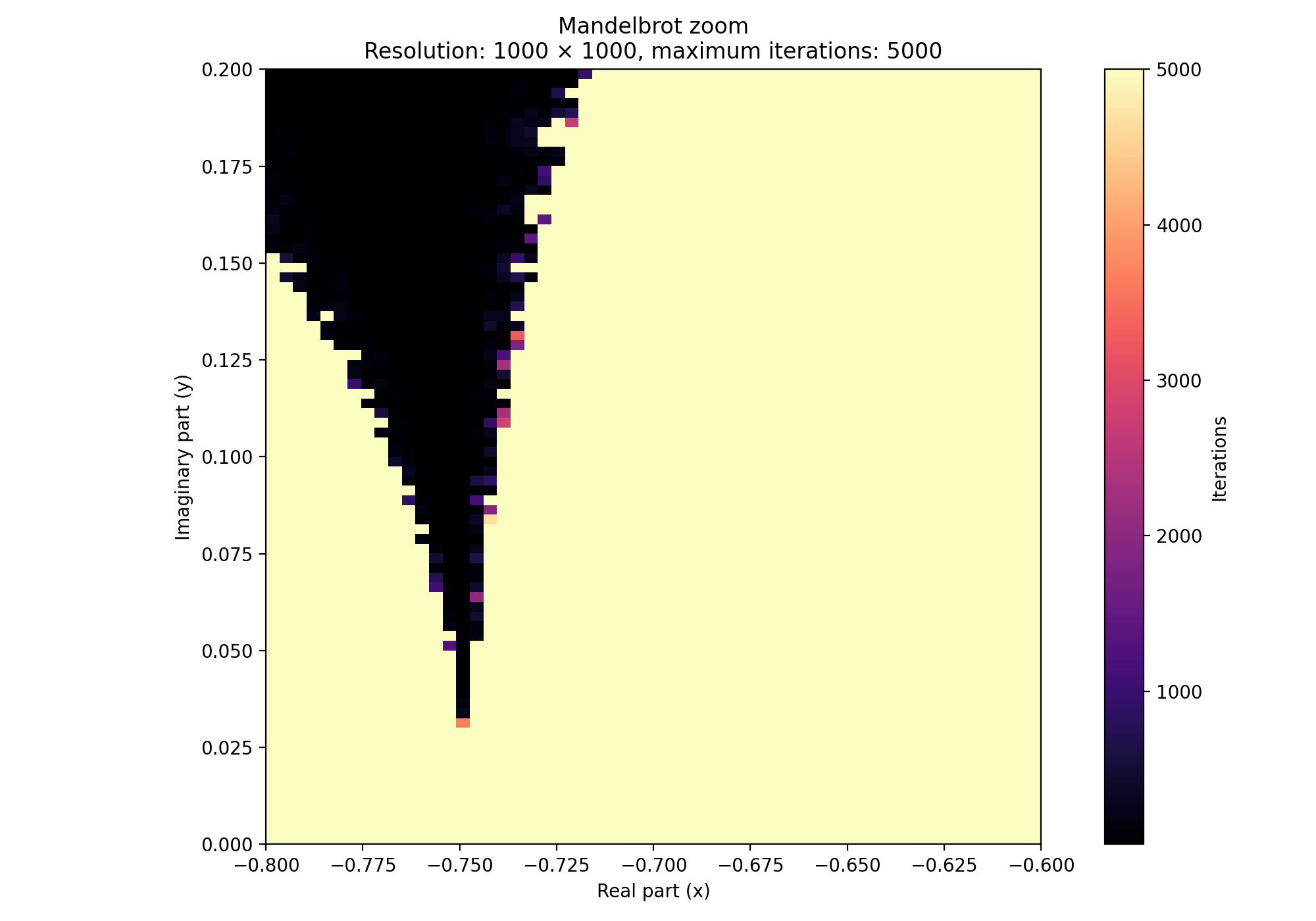
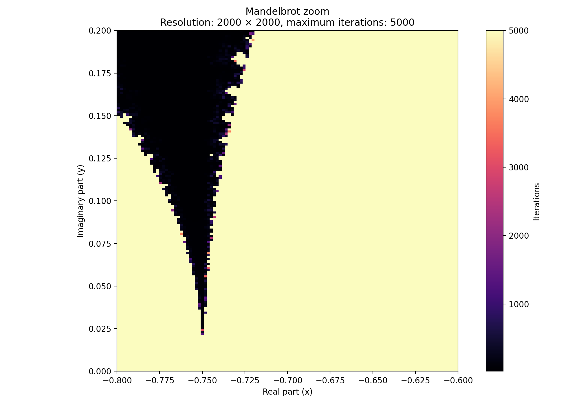
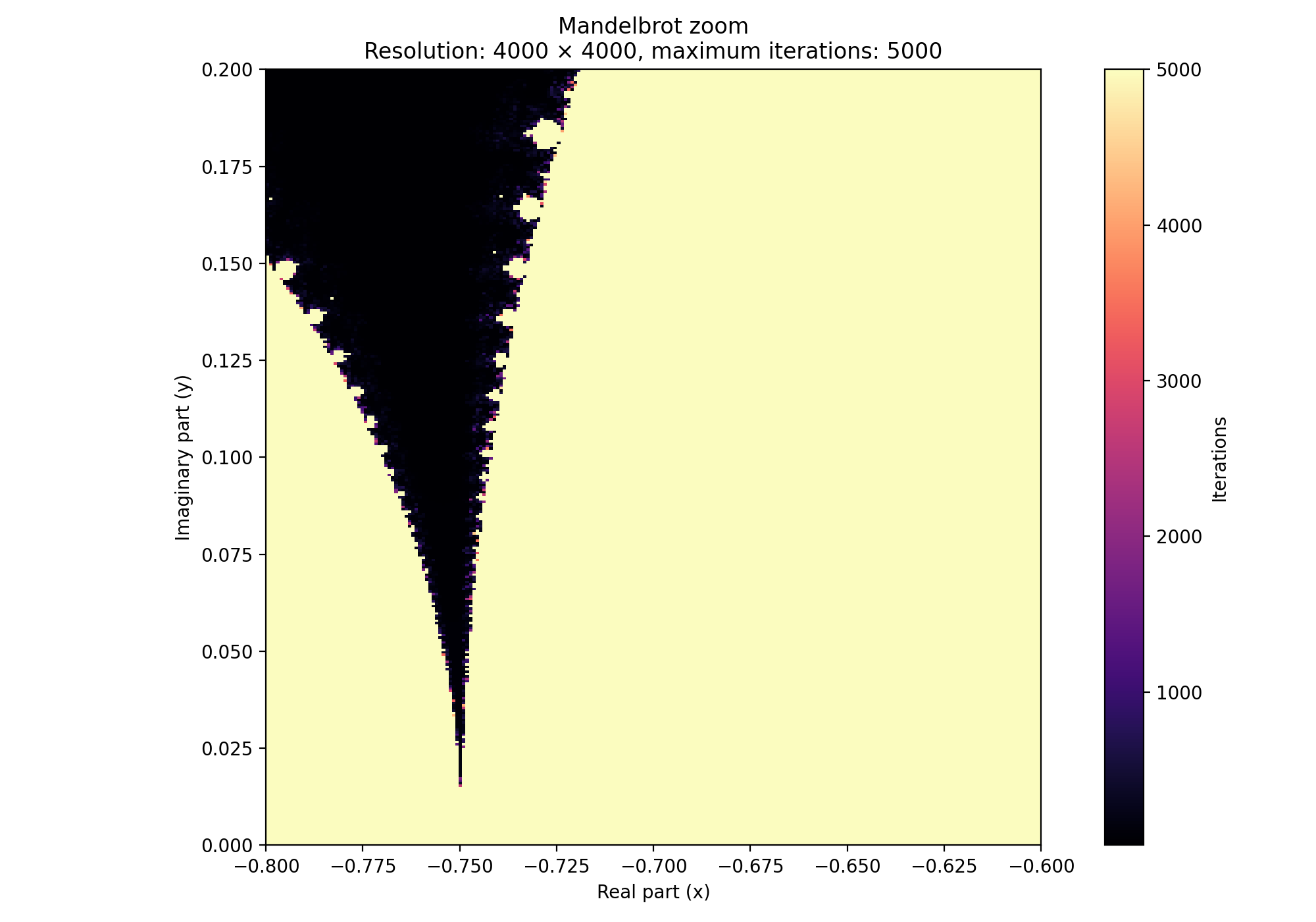
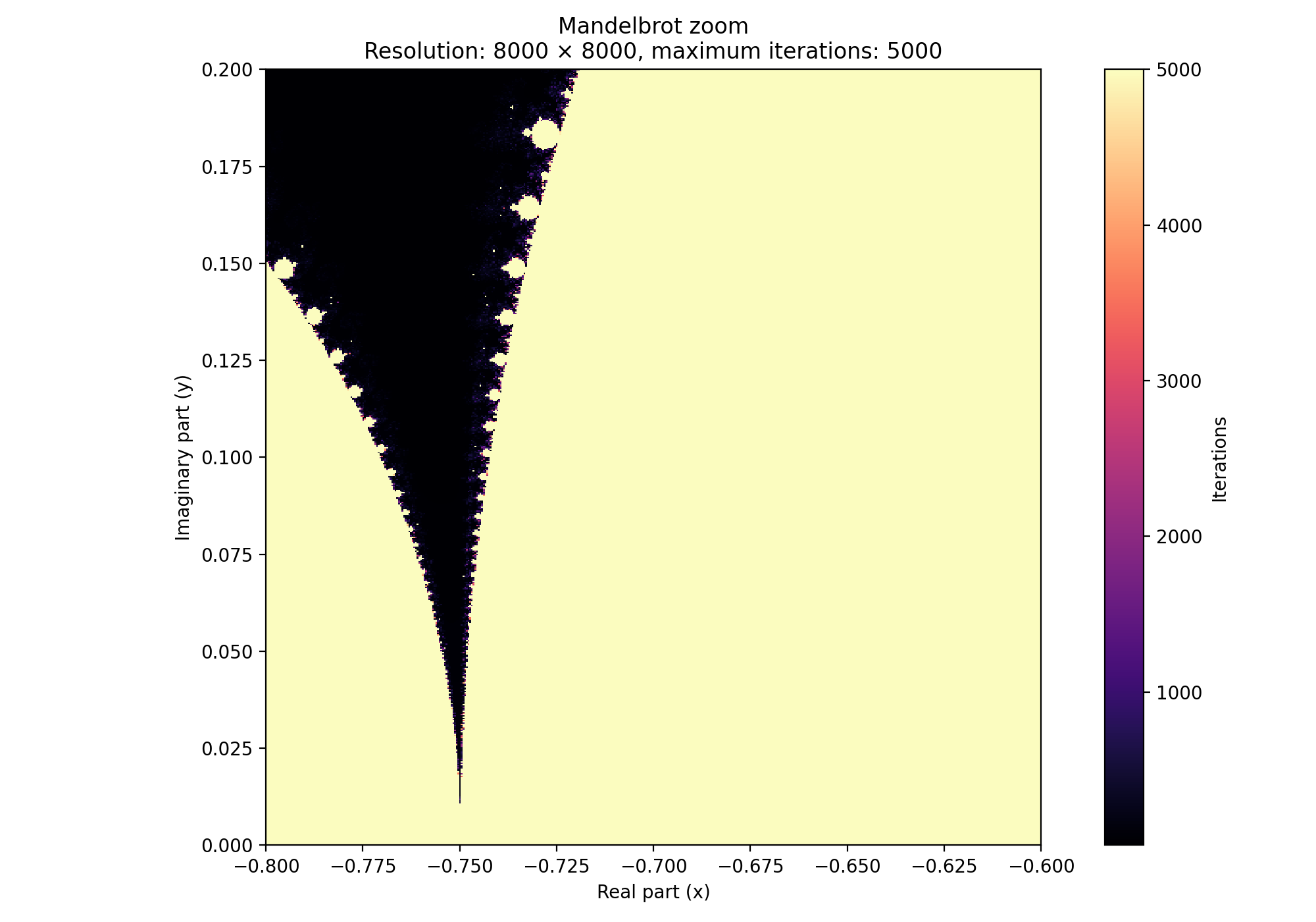
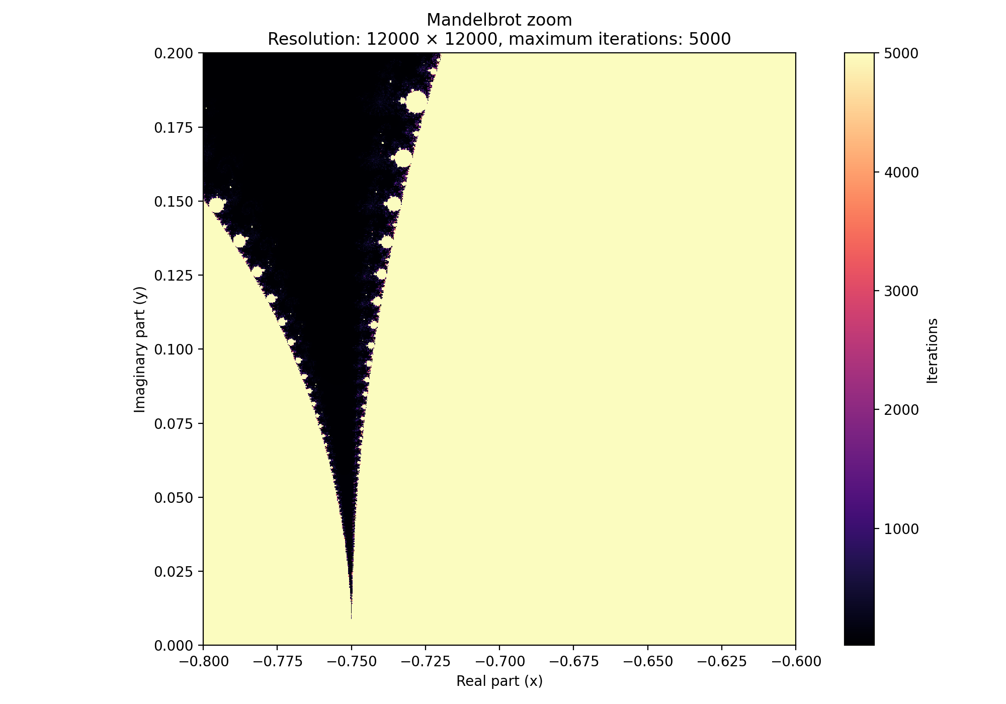
A run with a specified image dimension and iteration count produces a pixel-by-pixel binary file.

We convert this binary file into a png image using the visualization script.

python3 visualize.py image.bin

The visualization script extracts a small portion of the calculated image so that the effect of increasing resolution can be observed.

The visualization uses the fixed mathematical region

$$x=[-0.8,-0.6]$$

and

$$y=[0.0,0.2].$$

This is important.

If the mathematical coordinate range changes between images, comparisons can be misleading.

Keeping the same coordinate range means that increasing the resolution means adding more samples to the same mathematical region.

For example, the following images show the same zoom region at increasing resolutions.

1000 × 1000

2000 × 2000

4000 × 4000

8000 × 8000

12000 × 12000

As the resolution increases, more pixels are used to represent the same mathematical region.

10.1 Why Should the Serial, OpenMP, and CUDA Images Look the Same?

The purpose of parallelization is to change how the computation is executed, not what mathematical problem is being solved.

Ideally:

                    SAME MATHEMATICS
                           |
            +--------------+--------------+
            |              |              |
         Serial         OpenMP          CUDA
            |              |              |
            +--------------+--------------+
                           |
                           v
                       SAME RESULT

For the same:

• mathematical region;
• image resolution;
• maximum iteration count;
• Mandelbrot algorithm;

the three implementations should produce visually equivalent images.

The main difference should be how long the calculation takes.

Small numerical differences can occur near fractal boundaries because different processors and compilers may evaluate floating-point operations slightly differently. For this reason, “same result” should be understood as mathematically and visually equivalent rather than necessarily bit-for-bit identical.

The Mandelbrot calculation can be expressed as:

for each pixel:
    calculate pixel independently

This can be transformed into:

Serial

pixel 1 -> pixel 2 -> pixel 3 -> pixel 4 -> ...

OpenMP

thread 1 -> some pixels
thread 2 -> some pixels
thread 3 -> some pixels
...

CUDA

GPU thread 1 -> pixel 1
GPU thread 2 -> pixel 2
GPU thread 3 -> pixel 3
...
GPU thread many -> pixel many

This idea generalizes far beyond Mandelbrot.

When faced with a new computational problem, look for loops such as:

for (int i = 0; i < N; i++) {
    result[i] = f(data[i]);
}

Then ask:

Does calculating result[i] require information produced by result[i-1] or another iteration?

If the answer is no, there may be an opportunity for parallel execution.

For example:

result[0] = f(data[0])
result[1] = f(data[1])
result[2] = f(data[2])
...
result[N] = f(data[N])

can potentially be calculated concurrently.

This pattern occurs in:

• numerical integration;
• Monte Carlo methods;
• image processing;
• matrix operations;
• particle simulations;
• parameter sweeps;
• numerical PDE calculations;
• signal processing;
• statistical calculations.

The important point is not simply to ask:

“Can I use a GPU?”

Instead ask:

“Where is the independent work in my mathematical algorithm?”

12.1 OpenMP

OpenMP is often the easiest first step for an existing C/C++ program.

A suitable loop can frequently be parallelized with a directive such as:

#pragma omp parallel for

The program continues to use ordinary CPU memory.

Advantages

• relatively small programming change;
• uses existing CPU cores;
• good for large CPU-based workloads;
• suitable for many loops;
• easy to experiment with different thread counts.

Questions to consider

• Are the loop iterations independent?
• Are there race conditions?
• Is shared memory being accessed safely?
• How many threads should be used?
• Is the computation CPU-bound or memory-bound?
• Does performance continue to improve as more threads are added?

12.2 CUDA

CUDA requires a different execution model.

The programmer explicitly designs:

• GPU kernels;
• thread indexing;
• blocks;
• grids;
• device memory;
• CPU-GPU data transfers.

Advantages

• very large numbers of parallel threads;
• excellent for suitable data-parallel algorithms;
• particularly useful when the same operation is repeated over very large datasets.

Questions to consider

• Is the algorithm sufficiently parallel?
• How much data must be transferred to the GPU?
• Can the GPU remain busy?
• Is the calculation limited by GPU computation or memory bandwidth?
• What numerical precision is required?
• Is the extra programming complexity justified?

12.3 Which Approach Should I Use?

There is no universal rule that says every computation should use CUDA.

A useful first decision guide is:

This is only a starting point.

The best implementation depends on the structure of the algorithm, the amount of data, memory access patterns, numerical requirements, and the cost of moving data between different parts of the system.

The experiment also demonstrates an important practical issue.

Going from

$$1000\times1000$$

to

$$12000\times12000$$

does not mean that the problem became 12 times larger.

It became

$$12^2=144$$

times larger in terms of pixel count.

This is why high-resolution scientific calculations can become expensive very quickly.

Parallel computing makes it possible to explore larger resolutions and more computationally demanding parameter spaces within a practical time.

However, parallelism does not remove the computational cost. It changes how the available hardware is used to perform that work.

The Mandelbrot example suggests a general workflow.

                 Mathematical problem
                         |
                         v
                 Write a simple
                   serial program
                         |
                         v
                  Verify the result
                         |
                         v
               Identify independent work
                         |
                         v
                   Try OpenMP
                         |
                         v
                  Measure speedup
                         |
                         v
              Is the problem massively
                  data-parallel?
                    /          \
                  Yes           No
                   |             |
                   v             v
                 CUDA       Continue with CPU
                   |
                   v
              Measure again

A good principle is:

First make the mathematics correct. Then make the implementation parallel. Then measure.

This is preferable to starting with CUDA immediately.

A correct serial implementation is also extremely useful as a reference against which parallel implementations can be checked.

14.1 What to Look for in Your Own Code

When examining a research program, look for loops that perform the same calculation many times.

For example:

for (int i = 0; i < N; i++) {
    result[i] = expensive_function(data[i]);
}

Ask:

1. Is result[i] independent of result[j]?
2. Does each iteration perform a similar amount of work?
3. Is the number of iterations large?
4. Does each iteration access memory efficiently?
5. Is the computation dominated by arithmetic or by memory access?
6. Is there significant communication between iterations?
7. Does the calculation need to move data between CPU and GPU?

If the iterations are independent and there are many of them, OpenMP may be a good first experiment.

If there are very many similar independent calculations, CUDA may be worth considering.

If the calculation contains strong dependencies between iterations, forcing it into a massively parallel model may not help.

The Mandelbrot calculation is deliberately simple, but the programming ideas are broadly useful.

Lesson 1 — Hardware matters

Druta provides:

• 24 physical CPU cores;
• 48 logical processors;
• approximately 256 GB of RAM;
• an NVIDIA RTX 4500 Ada GPU with approximately 24 GB of GPU memory.

The resources available on the machine determine what types of computation can be explored efficiently.

Lesson 2 — Algorithms matter

The same mathematical problem can have very different execution characteristics depending on how it is programmed.

Lesson 3 — Parallelism matters

The Mandelbrot calculation contains a large amount of independent work.

That makes it suitable for:

• CPU multithreading with OpenMP;
• GPU parallelism with CUDA.

Lesson 4 — Measurement matters

Performance should be measured rather than assumed.

The fact that a machine has many cores or a powerful GPU does not by itself tell us how much faster a particular program will run.

Lesson 5 — Visualization helps

The Mandelbrot image provides an immediate way to check that the calculation is producing a meaningful result.

It also makes the effect of increasing resolution easy to see.

Lesson 6 — Scaling matters

Increasing resolution increases the number of calculations very rapidly.

For an $N\times N$ image, the number of pixels is proportional to $N^2$.

Lesson 7 — Match the problem to the hardware

The important idea is not that CUDA is always faster than OpenMP.

It is also not true that more CPU threads automatically make a program faster.

The important idea is:

Match the computational structure of the mathematical problem to the architecture of the machine.

The overall approach can be summarized as:

                  Mathematical problem
                          |
                          v
                  Understand the
                    computation
                          |
                          v
                  Find independent
                        work
                          |
             +------------+------------+
             |                         |
             v                         v
       CPU parallelism            GPU parallelism
             |                         |
             v                         v
          OpenMP                    CUDA
             |                         |
             +------------+------------+
                          |
                          v
                      Benchmark
                          |
                          v
                    Analyse result
                          |
                          v
                 Choose the approach
                 appropriate for the
                      real problem

The most useful skill to take away from this tutorial is therefore not specific knowledge of Mandelbrot, OpenMP, or CUDA.

It is the ability to look at a mathematical computation and ask:

Where is the independent work, and which part of Druta’s hardware is best suited to execute it?

That is the starting point for making effective use of a high-performance computing system.

• MATLAB 2025b
• g++
• gcc
• fort77
• conda 26.7.1
• System Python Version 3.14
• Conda Python Version 3.14
• FreeFem++
• FreeFem++-mpi
• FreeFem++-nw
• R 4.5.2
• nvcc: NVIDIA (R) Cuda compiler 12
• OpenMP 4.5
• links (For opening https://agnigarh.iitg.ac.in:1442/login?)
• jupyter-notebook
• Google Chrome
• Firefox
• htop

Open a terminal on your computer and execute the following command to connect to the Druta server. Replace username with your actual server username.

Note for Windows users: You may use Bitvise SSH Client or MobaXterm to connect to the server.

ssh -X username@172.16.68.3

Users are requested to create and use their own Conda environments instead of installing packages in the shared base environment.

After connecting to Druta, execute the following command to create a new environment:

user@druta:~$ conda create -n env_name python=3.13

Replace env_name with a name of your choice.

Note for TensorFlow users: If you plan to use TensorFlow, create an environment with Python 3.13, as TensorFlow compatibility depends on the Python version. Newer Python versions may not yet be supported by the TensorFlow release you intend to install.

After creating the environment, activate it using:

user@druta:~$ conda activate env_name

You may be prompted to log out of your shell after activating the environment. Please log out and log in to the server again.

Once the environment is activated, you will see the environment name at the beginning of your shell prompt:

(env_name) user@druta:~$

To check the Python version installed in your Conda environment, execute:

(env_name) user@druta:~$ python --version

You may need internet connection for installing a package. Open Firefox or Chrome browser for Internet connection:

(env_name) user@druta:~$ firefox

OR

(env_name) user@druta:~$ google-chrome

OR

(env_name) user@druta:~$ links https://agnigarh.iitg.ac.in:1442/login?

You can install Python packages using pip or conda within your Conda environment.

Note: Make sure your Conda environment is activated before installing packages. The active environment name should appear at the beginning of your shell prompt.

Using pip to install a single package:

(env_name) user@druta:~$ python -m pip install package_name

Using pip to install multiple packages:

(env_name) user@druta:~$ python -m pip install package1 package2 package3

Alternatively, using conda to install multiple packages:

(env_name) user@druta:~$ conda install package1 package2 package3

Replace package_name, package1, package2, and package3 with the names of the packages you require.

Important: Use python -m pip rather than simply pip to ensure that packages are installed using the Python interpreter associated with your active Conda environment.